Vertebrate Modeling
Overview
One of the major objectives of the National GAP Project is to document the representation of native vertebrate species in regional assesments. In order to meet this objective, we developed a spatial database of predicted species distributions throughout the region. While we don't have the resources to conduct a complete survey for every species, we do have access to a tremendous knowledge base that allows us to model distrubutions based on known range and habitat relationships.
The composition and structure of the dominant vegetation is an important and easily described measure of habitat for animals (Scott et al. 1993) and has long been used as an indirect indicator of animal distributions (Austin 1991). Other biotic and abiotic factors (i.e. elevation, wetland type, and distance from standing water) can also play a major role in defining a particular species' habitat. Many studies of vertebrate species have been conducted over the years documenting this type of information. In addition, data on known ranges for vertebrate species has also been collected. This includes not only survey data records, but the cumulative field experiences of biologists who work with these species on a daily basis. If we take a habitat description, break it down into vegetative communities and other environmental factors (e.g. elevation, wetland type, etc.), and then identified those areas within a known range, we would be creating a predicted distribution map. That is essentially what we did for each terrestrial vertebrate species modeled in the Southeast. The final step was to overlay those maps together to get a representation of biodiversity.
Why did we model only terrestrial vertebrates? Again, its a matter of resources. Realistically, we can only model a subset of all species. Terrestrial vertebrates are a logical choice because we generally know more about their habitat relationships and range extents than those of other taxa. Even so, there are over 600 terrestrial vertebrates modeled. The key to filling in the 'gaps' in the documented data is to have a thorough review by experts at every stage.
Return to Top
Species List Development
Selection Criteria
Gap Analysis predicted distribution maps are being created for all vertebrate species that breed in the Southeastern U.S. or use habitat there for an important part of their life history. Decisions were made on which species' habitats will be mapped based on standard Gap Analysis guidelines. Species lists have been created for each of the southeastern states by state-level Gap projects; these lists were compiled and pared down to remove some subspecies and domesticated species. Subspecies were only included when supported as distinct and non-overlapping with either the full species or other subspecies. The final list includes amphibians, mammals, reptiles, breeding birds, and wintering waterfowl.
Species Lists
After review, 602 species remained for habitat modeling:
Return to Top
Predictive Modeling of Habitat
Models of presence/absence for a species' predicted distribution may include a number of spatially explicit data sources. GAP models typically involve land use/land cover data as the primary input. However, other environmental features that make up the landscape constituting species' habitats can be valuable inputs to modeling. The SE-GAP project has attempted to use a number of data layers (ancillary data) other than land cover to develop species models. Many of these data layers act as surrogates for one or more aspects of a species' habitat that may only be inferred from available, remotely sensed information. The following document is meant to describe these data layers and their development, their range of parameters, and usage in modeling species' predicted distributions.
NOTE: The term "map unit" will be used throughout the document to mean the individual class or category mapped to represent land use and land cover, i.e. ecological systems.
Return to Top
Developing Known Range
All 602 terrestrial vertebrate species' geographic range extents were delineated as single or multiple polygons. Migratory species were primarily represented by breeding season ranges, however, wintering ranges for waterfowl and migratory bats were also delineated (33 species) Processes used to create range polygons were unique because information on the current geographic range of a species varies widely. However, a generalized approach used a variety of sources to develop species' ranges including sources of information in two broad categories: 1) species location records and range maps available digitally or in print, and 2) digital spatial data of environmental parameters described in later sections of this document.
Usage in Modeling
Species ranges were used as model delimiters in predicted distribution models.
Return to Top
Land Cover
Development
Ecological systems and land use mapped for the SE-GAP project are the primary input to species models. The development of these data is described in detail in subsequent documents. However, derivatives of these data were developed separately to further refine species models.
Primary and secondary (auxiliary) map units, and patch size (contiguous and non-contiguous patches) are parameters utilized as a model proceeds. That is, they are not stand-alone, independently created data layers. As such, they would not be considered "ancillary" data.
Usage in Modeling
Primary & Secondary Map Units
Primary map units are those land cover types critical for nesting, rearing young, and/or optimal foraging.
Secondary or auxiliary map units are those land cover types generally not critical for breeding, but are typically used in conjunction with primary map units for foraging, roosting, and/or sub-optimal nesting locations. These map units are selected only when located within a specified distance from primary map units.
Patch Size
The type and size of clusters of habitat can be assessed with spatial modeling. As a final step to the distribution modeling process, we used these parameters for species shown to require minimum amounts of habitat. This includes not only directly adjacent habitats, but those that are contextually adjacent. Both these parameters are utilized as the final step in a predicted distribution and therefore incorporate all other modeling inputs.
Contiguous Patch
Minimum Size (ha) - This parameter is set using the most conservative values explicitly stated in the literature. It applies only to the Southeastern portion of a species' range.
FROM Buffer - 0, 30, 60, 120, 250, 500, 1000 meters.
TO Buffer - 0, 30, 60, 120, 250, 500, 1000 meters.
Non-Contiguous Patch
The non-contiguous patch parameter is used to imply landscape context, i.e utilized habitats within a matrix of other habitats. It is measured as a percentage within a given area.
Forest & Edge Habitats
The edge or ecotone between forested and non-forested environments can be a critical aspect of the habitat landscape. We grouped map units into forested, non-forested, and shrubland/woodland land cover types to create unique data layers. These data layers can then be buffered at specified distances to identify species' habitats.
Development
All map units categorized as forest, non-forest, and shrubland/woodland were aggregated into separate data layers. Aggregated map units can be compared and contrasted to identify areas of transition between these broad categories. They can also be used to identify "core" areas or contiguous blocks of similar type (i.e. interior) through buffering procedures.
Forested map units were defined as those ecological systems and land uses that correspond to the National Land Cover Dataset (NLCD) forest/woodland classes (Homer et al. 2004) (Appendix A). These included NLCD classes "deciduous forest", "evergreen forest", "mixed forest", "palustrine forested wetland", and "estuarine forested wetland" (class values 41, 42, 43, 91 and 93 respectively). Non-forested map units were defined as those ecological systems and land uses not categorized as forest using the criteria stated above. Woodland/shrubland map units were defined as those ecological systems and land uses containing a majority of short, scrubby, woody vegetation or sparsely canopied treed vegetation (Appendix B). Unlike the forested map units, the woodland/shrubland layer was not explicitly derived from NLCD classes but was selected individually based on attributes defined by the systems and land uses.
Once these data layers were created, buffering procedures created unique datasets containing unique categories of distance: > 4000, 4000, 2000, 1000, 500, 250, 120, 60, and 30 meters into and away from the specified feature.
Usage in Modeling
Forest Interior
This data layer constitutes unique aggregations of forest and non-forest map units. Non-forest map units include water, pasture/hay, agricultural areas, urban/developed, marshes, beaches, etc...
Utilizes Forest Interior - For species that require interior forest. Buffer distances must be identified to utilize this input.
Avoids Forest Interior - For species that avoid interior forest. Buffer distances must be identified to utilize this input.
FROM Buffer - 0, 30, 60, 120, 250, 500, 1000, 2000, 4000, and 9999 (> 4000 m) (Figure 1.)
INTO Buffer - 0, 30, 60, 120, 250, 500, 1000, 2000, 4000, and 9999 (> 4000 m) (Figure 1.)
Edge/Ecotone Type & Width
Forest/Open Ecotone Only - This data layer represents the transitional areas between forest and open, non-forested habitats. Open, non-forested habitats include water, pasture/hay, prairies, agricultural areas, urban/developed, marshes, beaches, etc...
Forest/Open Ecotone + Woodlands/Shrublands - The forest/open only ecotone does not consider environments with sparse canopies or scrubby vegetation. In order to account for these additionally complex ecotones, this data layer includes woodland and shrubland map units that would otherwise be ignored.
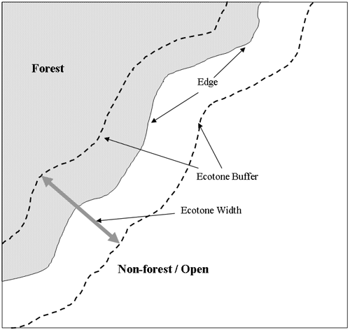
Ecotone Width - This distance represents a swath of symmetrically buffered edge. The parameter is measured in increments of 0, 30, 60, 120, 250, 500, and 1000 meters. For example, an ecotone width of 500 meters includes 250 meters into forest and 250 meters into open (Figure 1).
Figure 1. Example of an ecotone/edge buffer on forest/non-forested environments.

Return to Top
Hydrologic Unit Codes (HUCs)
Development
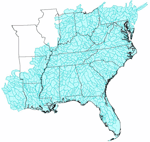
The HUC is part of a hierarchical classification system for surface water drainage in the US (Seaber et al. 1987). The numerical code represents a "cataloging unit" of delineation approximately larger than 1800 square kilometers. Within the SE-GAP project boundary there are 577 8-digit HUCs (Figure 2). Vector format (i.e. polygon) data were compiled from United States Geological Survey (USGS) sources. No ancillary data was produced directly from HUCs, but they were utilized in numerous other ancillary data layer processes. Most notably, HUCs allow for partitioned processing when scripting complex spatial analysis tasks.
Figure 2. The 577 8-digit HUCs in the SE-GAP project region.

Usage in Modeling
HUCs were not used directly in species modeling. However, some species' geographic ranges were developed using the 8-digit hydrologic unit code polygons. This was only appropriate for species whose ranges would conceivably be limited to certain watershed drainages and their associated topographic distinctions. In most cases, these species were partially or entirely aquatic during some part of their life history (e.g. salamanders, turtles).
Return to Top
Ecoregions
Development
Ecoregions developed by Omernik (1987, 1995) and available from the U.S. Environmental Protection Agency (US EPA 2007) were produced through an analysis of biotic and abiotic patterns relating to ecosystem differentiation. Although no ancillary date were created directly from ecoregions, they were utilized in numerous other primary and ancillary data layer processes including land cover/ecological systems, species' ranges, and landforms.
Usage in Modeling
Ecoregions were not used explicitly in predicted distribution models. However, Omernik Level III and Level IV ecoregions were used to help define polygon boundaries for some species' geographic ranges when appropriate. Some species are clearly restricted to the physiographic and geographic patterns and boundaries that ecoregions define. For these species, ecoregions were used as all or a portion of the polygon(s) delineation. If there was a doubt as to the limitations imposed by such boundaries, ecoregions were not used.
Return to Top
Soils
Development
State geographic soils database (STATSGO) soil units polygons were developed by the U.S. Department of Agriculture's Natural Resource Conservation Service (NRCS) at a scale of 1:250,000 for the conterminous U.S. (USDA 1995). Although no ancillary date were created directly from soils, they were utilized in numerous other primary and ancillary data layer processes including land cover/ecological systems, species' ranges, and landforms.
Usage in Modeling
Soils were not used explicitly in predicted distribution models. However, soils were used to help define polygon boundaries for some species' geographic ranges when appropriate. Although ecoregions consider soils as an abiotic factor in their delineation, for certain species it was necessary to focus more narrowly on soil type to help define a range polygon. For species whose habitat requirements are restricted to certain soil types (particularly some reptiles), soil polygons were used to help delineate all or a portion of their range.
Return to Top
Roads
Development
Roads data were compiled from the U.S. Census Bureau's TIGER/Line files (USCB 2007). As a preliminary and stand alone layer, road density grids were created so that they could be used for production of imperious surface data layers and, by proxy, land cover/land use map units, as well as in production of an avoidance mask for vertebrate modeling. Part of the procedure to develop road density required the summarization of the attribute code 'CFCC' within the TIGER database (see technical documentation for TIGER/Line files at the URL listed in the Literature Cited section for more information). In general, seven codes were combined into three road category types (Table 1). A line density algorithm was used to calculate the linear length of roads within a circular neighborhood. The algorithm utilized a kernel smoothing function on a 30 meter cell size within a 564.19 meter radius (1 km2).
| Table 1. TIGER/Line attribute codes and descriptions and corresponding SE-GAP summarized categories used to develop road density for the southeast region. |
| Code Description |
CFCC Code |
SE-GAP Category |
| Primary highway with limited access | A1 | US Highway |
| Primary road without limited access | A2 | State Route |
| Secondary and connecting road | A3 | State Route |
| Local, neighborhood, and rural road | A4 | Secondary |
| Vehicular trail | A5 | Secondary |
| Roads with special characteristics | A6 | Secondary |
| Road as thoroughfare | A7 | Secondary |
Usage in Modeling
Roads were not used explicitly in predicted distribution models. However, the road density data layer derived from roads was used to develop an avoidance mask as an index to human disturbance (see Urban).
Return to Top
Elevation
Development
Elevation data are often represented in digital elevation models (DEMs). SE-GAP utilized the USGS compiled National Elevation Dataset (NED) as a primary source (USGS 2003). However, because of the varying quality of the data, it was necessary to incorporate other datasets to create an improved, region wide product. These included data from NASA's Shuttle Radar Topography Mission (SRTM) at 30 meter resolution (NASA 2007), Light Detection and Ranging (LIDAR) data from the North Carolina Floodplain Mapping Program (NCFMP 2007), and hypsography data from the USGS's Digital Line Graphs (DLGs) at 1:24,000 and 1:100,000 scales (USGS 2007a). Areas of inconsistent, erroneous, or systematically flawed data were identified visually and "tagged" for fixing. A number of algorithms were then used to reassign elevation values using interpolations based on the higher quality data. This essentially promoted the best available information for a given area using a number of sources, as opposed to re-interpolating data from the same flawed source.
Usage in Modeling
Some species respond to environments directly related to altitudinal variation. Elevation is easily implemented in spatial modeling by limiting the model to the minimum and maximum values explicitly stated in the literature. DEMs are utilized directly and are measured in meters above mean sea level.
Return to Top
Land Forms
Development
Landforms are derived from DEMs, ecoregions and hydrography using a complex model of slope, aspect, location, elevation, flow direction and accumulation, and a variety of other interpolated data. These are meant to incorporate a mixture of environmental inputs important for species.
The general steps involved in creating landforms are as follows:
- Extract data inputs for a given region to process (mapping zones for example).
- Subdivide into smaller processing units (HUCs for example) that can be overlapped during iteration loops to facilitate merging during production of the final output.
- Calculate Topographic Relative Moisture Index (TRMI) based on a DEM and hydrography. TRMI is an estimate of potential moisture at a specific location created by combining relative slope position, aspect, slope and curvature from the DEM, and defining valley bottoms that correspond to high resolution hydrography data.
- Process the moisture index grid to reclassify it into binary categories of moist and dry; smoothing the output with a majority filter to remove single cells and linear artifacts.
- Calculate land position based on the inverse distance weighted elevation of each cell in relation to its neighbors.
- Calculate the landform for each processing unit by combining the moisture, land position, slope and aspect.
- Create the final landform for the region by combining landforms of overlapping processing units into a single output.
Usage in Modeling
Species distributions are restricted to the selected landforms. Landforms include:
Cliffs, Steep Slopes, Slope Crests, Side Slopes, Upper Slopes, Flat Summits, Coves, Slope Bottoms, Moist Flats, Dry Flats, and Wet Flats.
Return to Top
Hydrography
Development
Water and its location on the landscape is a very important aspect of species' habitats. SE-GAP used a number of water related data layers to refine species models. These include water type (i.e. flowing or open/standing), distance to and from water, and stream flow and underlying gradient.
The source for hydrographic data was the USGS National Hydrography Dataset (NHD)(USGS 2007b). The NHD is composed of the most up-to-date nationwide data of surface waters compiled at two scales: 1:24,000 and 1:100,000. SE-GAP began acquiring NHD data in 2003. At the time, NHD was available only in ArcInfo coverage format organized by 8-digit Hydrologic Unit Code (HUC). NHD 8-digit HUCs are a complex mixture of polygon and arc (and point) features with numerous related tables of attributes. These coverage data are vector data types, i.e. arcs, polygons, nodes etc. with their incumbent data tables.
Water Type
We divided hydrographic features from NHD into three types: flowing water, standing water, and wet vegetation. These feature types were extracted from the NHD by selecting corresponding codes (the FCODE attribute) in data tables and creating separate datasets for each data type. To facilitate their use in spatial modeling, these feature types were converted to grids and combined into 16 categories where feature types overlapped (Table 2).
Flowing Water -
Flowing water represents hydrographic features such as streams, rivers, springs, etc... NHD was developed as a value added product to allow users to performing tasks such as routing, classification, segmentation, etc... Therefore, arcs which flow into waterbodies such as reservoirs need to be continuous from their origin to their terminus. These "connectors" or "artificial paths" were also extracted from the data to represent flowing water. Flowing water can be arc or polygon feature classes. This is particularly true for large rivers that are wide enough to be digitized as long, narrow polygons.
Standing Water -
Standing water represents hydrographic features such as lakes, ponds, reservoirs, bays, inlets, etc... Standing water can be arc or polygon feature classes. Some canals and ditches are represented as arcs. However, most standing water features are polygons.
Wet Vegetation -
Wet vegetation represents hydrographic features such as swamps, marshes, Carolina bays, etc... It is represented only as the polygon feature class.
| Table 2. Grid cell values for NHD hydrographic features assembled by 8-digit HUC. |
| Basic Featues |
| Grid Cell Value |
Description |
| 0 | No Features |
| 1 | Flowing Water Arcs |
| 2 | Flowing Water Polygons |
| 4 | Standing Water Arcs OR Standing Water Ploygons |
| 8 | Wet Vegetation |
| Combination of Featues |
| Grid Cell Value |
Description |
| 3 | Flowing Water Arcs & Polygons |
| 5 | Flowing Water Arcs AND {Standing Water Arcs OR Standing Water Polygons} |
| 6 | Flowing Water Polygons AND {Standing Water Arcs OR Standing Water Polygons} |
| 7 | Flowing Water Arcs & Polygons AND Standing Water Arcs & Polygons |
| 9 | Flowing Water Arcs AND Wet Vegetation |
| 10 | Flowing Water Polygons AND Wet Vegetation |
| 11 | Flowing Water Arcs & Polygons AND Wet Vegetation |
| 12 | {Standing Water Arcs OR Standing Water Polygons} AND Wet Vegetaton |
| 13 | Flowing Water Arcs AND {Standing Water Arcs OR Standing Water Polygons} AND Wet Vegetation |
| 14 | Flowing Water Polygons AND {Standing Water Arcs OR Standing Water Polygons} AND Wet Vegetation |
| 15 | All Types of Hydro |
Distance INTO and FROM Water Features
We used 18 categories of distance from the water features flowing water, standing water and wet vegetation. A process was used to buffer hydrography at various distances and code grid cells based on a defined set of distances. Table 3 summarizes the 18 code categories for buffer grids. Each water type has a region wide grid coded for buffer distance from that type of hydrography.
| Table 3. Coding for 18 unique categories of buffer distance from hydrography. |
| Exterior Buffers (from feature) |
| Cell Value |
Buffer Distance from Hydrographic Feature (meters) |
| 0 | > 4000m |
| 1 | +2000m to +4000m |
| 2 | +1000m to +2000m |
| 3 | +500m to +1000m |
| 4 | +250m to +500m |
| 5 | +120m to +250m |
| 6 | +60m to +120m |
| 7 | +30m to +60m |
| 8 | 0m to +30m |
| Interior Buffers (into feature) |
| Cell Value |
Buffer Distance from Hydrographic Feature (meters) |
| 9 | 0m to -30m |
| 10 | -30m to -60m |
| 11 | -60m to -120m |
| 12 | -120m to -250m |
| 13 | -250m to -500m |
| 14 | -500m to -1000m |
| 15 | -1000m to -2000m |
| 16 | -2000m to -4000m |
| 17 | > 4000m |
Velocity (Stream Gradient)
Stream velocity (or more appropriately stream gradient) was derived from a combination of streams and slopes calculated from a digital elevation model (DEM). A process was developed that determined the cell-to-cell drop in elevation along a stream grid based on flow direction. The process created three categories of slope calculations for use as a surrogate for stream gradient/velocity (Table 4). A double pass focal majority function was used to "smooth" the output.
| Table 4. Coding for 3 unique categories of stream slope / gradient and corresponding velocity surrogate. |
| Cell Value |
Cell-to-Cell Slope (degrees) |
Cell-to-Cell Slope (%) |
Assumed Velocity |
| 0 | <= 0 | 0 | Slow |
| 1 | 0 - 3 | 0 - 5.2 | Moderate |
| 2 | >= 3 | > 5.2 | Fast |
Usage in Modeling
Water Type
Flowing Water - This includes streams, rivers, springs, seeps, ditches with moving water etc...
Open/Standing Water - This includes bays, estuaries, ocean, lakes, ponds, reservoirs, ditches with stagnant water etc...
Wet Vegetation - This includes a collection of map units representing seasonally or tidally inundated woody and non-woody plants.
Distance INTO and FROM Water Features
Interior (INTO) and Exterior (FROM) buffers on water features measured in meters and represented as discrete, cumulative distances. For example, a 250 meter exterior buffer on flowing water includes all areas up to 250 meters from the flowing water feature.
FROM Buffer - 0, 30, 60, 120, 250, 500, 1000, 2000, 4000, and 9999 (> 4000 m)
INTO Buffer - 0, 30, 60, 120, 250, 500, 1000, 2000, 4000, and 9999 (> 4000 m)
Velocity (Stream Gradient)
For some aquatic species, this can represent an important aspect of their habitat such as oxygenation levels, presence of invertebrate prey, and amount of sediment within the water column and on streambed substrates.
Slow Only - For species that require slow moving or almost stagnant sections of streams or rivers. Typically these are areas where the underlying topography is flat (0 % gradient).
Fast Only - For species that require high velocity sections of streams or rivers. Typically these are areas where the underlying topography is steep. A threshold of > 5 % gradient was used.
All Types - Species can utilize either fast or slow sections of streams or rivers.
Return to Top
Salinity
Development
Water salinity is a major factor when considering habitat conditions for many species. However, the dynamic and complex nature of water systems makes the development of a highly refined and reliable datalayer impractical, if not impossible. Therefore, we developed three general categories to include in species habitat models.
Zones of water salinity were hand digitized using NLCD map units as a guide. All palustrine and upland map units were identified, as were all estuarine map units. A line was digitized between non-estuarine and estuarine map units and served as the boundary between fresh and brackish water. An additional line was digitized across all ocean inlets, essentially the shortest distance between two bodies of land. This second line served as the boundary between brackish and salt water.
Usage in Modeling
Freshwater Only - For species requiring water, this includes only fresh water.
Brackish/Salt Water Only - For species requiring water, this includes only brackish/salt water.
All Water - For species requiring water, this includes both brackish/salt water as well as freshwater.
Return to Top
Urban Environments
Development
Environments dominated by human disturbance such as roads, cities, and the constructed materials that support human habitation have profound effects on species' distributions. Map units derived for SE-GAP include three categories of development intensity - high, medium and low. These classes rely on spectral signatures from satellite data in association with measurements of impervious surface. SE-GAP created an urban/avoidance data layer using a combination of road density (see Roads section above) and the three map units of development intensity. In effect, the derived data layer acts as an index for a species' intolerance to human environments.
Usage in Modeling
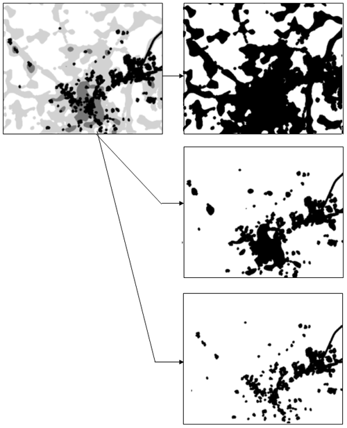
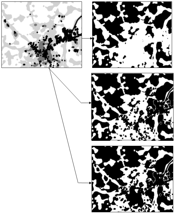
For most species, this data layer was used to "mask out" or exclude species from a portion of the landscape (see Figure 3). However, some species respond favorably to human habitats. In this later case, the data layer was used in an inclusionary manner see (Figure 4).
Level of Tolerance/Intolerance
This parameter is ranked at three levels: high, medium, and low. No selection of this parameter indicates the species' model is not contingent on an index of human disturbance.
High -
Exclusionary - For species that are very intolerant of human disturbance. All portions of the landscape identified as being directly influenced by human disturbance are eliminated from the predicted distribution.
Inclusionary - For species that are associated with high levels of human disturbance. The predicted distribution is limited to all portions of the landscape identified as being directly influenced by human disturbance.
Medium -
Exclusionary - For species that are moderately intolerant of human disturbance. Only portions of the landscape identified as being highly or moderately influenced by human disturbance are eliminated from the predicted distribution.
Inclusionary - For species that are associated with moderate levels of human disturbance. The predicted distribution is limited to only portions of the landscape identified as being moderately or partially influenced by human disturbance.
Low -
Exclusionary - For species that are partially intolerant of human disturbance. Only portions of the landscape identified as being highly influenced by human disturbance are eliminated from the predicted distribution.
Inclusionary - For species that are associated with partial levels of human disturbance. The predicted distribution is limited to only portions of the landscape identified as being partially influenced by human disturbance.
Figure 3. The index of human disturbance at three levels: light gray = low; gray = medium; black = high. Using an exclusionary mask, the predicted distribution of a species is excluded from the black areas and limited to the white areas at intolerance levels of high, medium and low (top to bottom).

Figure 4. The index of human disturbance at three levels: light gray = low; gray = medium; black = high. Using an inclusionary mask, the predicted distribution of a species is excluded from the black areas and limited to the white areas at tolerance levels of high, medium and low (top to bottom).

Return to Top
Literature Cited
Austin, M.P. 1991. Vegetation: data collection and analysis. Pages 37-41 in C.R. Margules and M.P. Austin, eds. Nature conservation: cost effective biological surveys and data analysis. Australia CSIRO, East Melbourne.
Homer, C. C. Huang, L. Yang, B. Wylie and M. Coan. 2004. Development of a 2001 National Landcover Database for the United States. Photogrammetric Engineering and Remote Sensing, Vol. 70, No. 7, July 2004, pp. 829-840.
National Aeronautics and Space Administration. 2007. Jet Propulsion Laboratory, Califorinia Institute of Technology. Shuttle Radar Topography Mission. Available online, URL: http://www2.jpl.nasa.gov/srtm/.
North Carolina Floodplain Mapping Program. 2007. North Carolina Floodplain Mapping Information System. Available online, URL: http://www.ncfloodmaps.com/.
Omernik, J.M. 1987. Ecoregions of the conterminous United States. Map (scale 1:7,500,000). Annals of the Association of American Geographers 77(1):118-125.
Omernik, J.M. 1995. Ecoregions: A spatial framework for environmental management. In: Biological Assessment and Criteria: Tools for Water Resource Planning and Decision Making. Davis, W.S. and T.P. Simon (eds.) Lewis Publishers, Boca Raton, FL. Pp. 49-62.
Scott, M., F. Davis, B. Csuti, R. Noss, B. Butterfield, C. Groves, H. Anderson, S. Caicco, F. D'Erchia, T.C. Edwards Jr., J. Ulliman and R.G. Wright. 1993. Gap Analysis: A geographic approach to protection of biological diversity. Wildlife Monographs, no. 123. The Journal of Wildlife Management. 57(1) 41pp.
Seaber, P.R., Kapinos, F.P., and Knapp, G.L., 1987, Hydrologic Unit Maps: U.S. Geological Survey Water-Supply Paper 2294, 63 p.
U.S. Census Bureau. 2007. Topologically Integrated Geographic Encoding and Referencing system. Available online, URL: http://www.census.gov/geo/www/tiger/. Documentation available online, URL: http://www.census.gov/geo/www/tiger/tiger2006se/TGR06SE.pdf.
U.S. Department of Agriculture. 1995. State soil geographic (STATSGO) data base, data use information. NRCS National Soil Survey Center Miscellaneous Publication # 1492. Available on, URL: http://www.nrcs.usda.gov/technical/techtools/statsgo_db.pdf.
U.S. Environmental Protection Agency. 2007. Western Ecology Division, Corvallis, OR. Ecoregion Maps and GIS Resources. Available online, URL: http://www.epa.gov/wed/pages/ecoregions.htm.
U.S. Geological Survey. 2003. National Mapping Division EROS Data Center. National Elevation Dataset. Available online, URL: http://ned.usgs.gov/.
U.S. Geological Survey. 2007a. National Mapping Division EROS Data Center. Digital Line Graphs. Available online, URL: http://eros.usgs.gov/products/map/dlg.html.
U.S. Geological Survey. 2007b. National Hydrography Dataset. Available online, URL: http://nhd.usgs.gov/index.html.
Return to Top
Appendix A
| Table of forested map units (ecological system) corresponding to National Land Cover Dataset (NLCD) classes. |
| Ecological System Group Name |
NLCD Class Name |
NLCD Class Value |
| Southern Piedmont Dry Oak-Heath Forest - Hardwood Modifier |
DECIDUOUS FOREST/WOODLAND |
41 |
| Southern Piedmont Dry Oak-Heath Forest - Virginia/Pitch Pine Modifier |
EVERGREEN FOREST/WOODLAND |
42 |
| Southern Piedmont Dry Oak-Heath Forest - Mixed Modifier |
MIXED FOREST/WOODLAND |
43 |
| Central and Southern Appalachian Spruce-Fir Forest |
EVERGREEN FOREST/WOODLAND |
42 |
| Central and Southern Appalachian Northern Hardwood Forest |
DECIDUOUS FOREST/WOODLAND |
41 |
| Southern Piedmont Seepage Wetland |
PALUSTRINE FORESTED WETLAND |
91 |
| Southern Piedmont Small Floodplain and Riparian Forest |
PALUSTRINE FORESTED WETLAND |
91 |
| Southern Piedmont Large Floodplain Forest - Forest Modifier |
PALUSTRINE FORESTED WETLAND |
91 |
| Southern Appalachian Low Mountain Pine Forest |
EVERGREEN FOREST/WOODLAND |
42 |
| Southern Piedmont/Ridge and Valley Upland Depression Swamp |
PALUSTRINE FORESTED WETLAND |
91 |
| Southern Piedmont Dry Oak-(Pine) Forest - Hardwood Modifier |
DECIDUOUS FOREST/WOODLAND |
41 |
| Southern Piedmont Dry Oak-(Pine) Forest - Loblolly Pine Modifier |
EVERGREEN FOREST/WOODLAND |
42 |
| Southern Piedmont Dry Oak-(Pine) Forest - Mixed Modifier |
MIXED FOREST/WOODLAND |
43 |
| Southern Piedmont Mesic Forest |
DECIDUOUS FOREST/WOODLAND |
41 |
| Allegheny-Cumberland Dry Oak Forest and Woodland |
DECIDUOUS FOREST/WOODLAND |
41 |
| Allegheny-Cumberland Dry Oak Forest and Woodland - Hardwood Modifier |
DECIDUOUS FOREST/WOODLAND |
41 |
| Allegheny-Cumberland Dry Oak Forest and Woodland - Pine Modifier |
EVERGREEN FOREST/WOODLAND |
42 |
| Southern and Central Appalachian Cove Forest |
DECIDUOUS FOREST/WOODLAND |
41 |
| Southern Ridge and Valley Dry Calcareous Forest |
DECIDUOUS FOREST/WOODLAND |
41 |
| Southern Ridge and Valley Dry Calcareous Forest - Pine Modifier |
EVERGREEN FOREST/WOODLAND |
42 |
| Southern Ridge and Valley Dry Calcareous Forest - Hardwood Modifier |
DECIDUOUS FOREST/WOODLAND |
41 |
| Southern Piedmont Northern Triassic Basin Dry Forest |
DECIDUOUS FOREST/WOODLAND |
41 |
| Central Appalachian Oak and Pine Forest |
MIXED FOREST/WOODLAND |
43 |
| Northeastern Interior Dry Oak Forest-Hardwood Modifier |
DECIDUOUS FOREST/WOODLAND |
41 |
| Northeastern Interior Dry Oak Forest - Virginia/Pitch Pine Modifier |
EVERGREEN FOREST/WOODLAND |
42 |
| Northeastern Interior Dry Oak Forest - Mixed Modifier |
MIXED FOREST/WOODLAND |
43 |
| Appalachian Hemlock-Hardwood Forest |
MIXED FOREST/WOODLAND |
43 |
| Central and Southern Appalachian Montane Oak Forest |
DECIDUOUS FOREST/WOODLAND |
41 |
| North-Central Appalachian Acidic Swamp |
PALUSTRINE FORESTED WETLAND |
91 |
| North-Central Interior and Appalachian Rich Swamp |
PALUSTRINE FORESTED WETLAND |
91 |
| Central Appalachian Floodplain - Forest Modifier |
PALUSTRINE FORESTED WETLAND |
91 |
| Central Appalachian Riparian - Forest Modifier |
PALUSTRINE FORESTED WETLAND |
91 |
| South-Central Interior Large Floodplain - Forest Modifier |
PALUSTRINE FORESTED WETLAND |
91 |
| South-Central Interior Small Stream and Riparian |
PALUSTRINE FORESTED WETLAND |
91 |
| Southern and Central Appalachian Oak Forest |
DECIDUOUS FOREST/WOODLAND |
41 |
| South-Central Interior Mesophytic Forest |
DECIDUOUS FOREST/WOODLAND |
41 |
| South-Central Interior Highlands Dry Oak Forest |
DECIDUOUS FOREST/WOODLAND |
41 |
| Atlantic Coastal Plain Northern Mixed Oak-Heath Forest |
DECIDUOUS FOREST/WOODLAND |
41 |
| Mississippi River Riparian Forest |
PALUSTRINE FORESTED WETLAND |
91 |
| Mississippi River Low Floodplain (Bottomland) Forest |
PALUSTRINE FORESTED WETLAND |
91 |
| Atlantic Coastal Plain Southern Tidal Wooded Swamp |
ESTUARINE FORESTED WETLAND |
93 |
| Atlantic Coastal Plain Dry and Dry-Mesic Oak Forest |
DECIDUOUS FOREST/WOODLAND |
41 |
| Atlantic Coastal Plain Mesic Hardwood and Mixed Forest |
DECIDUOUS FOREST/WOODLAND |
41 |
| Atlantic Coastal Plain Clay-Based Carolina Bay Forested Wetland |
PALUSTRINE FORESTED WETLAND |
91 |
| Atlantic Coastal Plain Blackwater Stream Floodplain Forest - Forest Modifier |
PALUSTRINE FORESTED WETLAND |
91 |
| Atlantic Coastal Plain Brownwater Stream Floodplain Forest |
PALUSTRINE FORESTED WETLAND |
91 |
| Atlantic Coastal Plain Small Blackwater River Floodplain Forest |
PALUSTRINE FORESTED WETLAND |
91 |
| Atlantic Coastal Plain Small Brownwater River Floodplain Forest |
PALUSTRINE FORESTED WETLAND |
91 |
| Southern Coastal Plain Nonriverine Cypress Dome |
PALUSTRINE FORESTED WETLAND |
91 |
| Atlantic Coastal Plain Fall-Line Sandhills Longleaf Pine Woodland - Loblolly Modifier |
EVERGREEN FOREST/WOODLAND |
42 |
| Atlantic Coastal Plain Fall-line Sandhills Longleaf Pine Woodland - Offsite Hardwood Modifier |
DECIDUOUS FOREST/WOODLAND |
41 |
| Atlantic Coastal Plain Central Maritime Forest |
EVERGREEN FOREST/WOODLAND |
42 |
| Atlantic Coastal Plain Northern Tidal Wooded Swamp |
ESTUARINE FORESTED WETLAND |
93 |
| East Gulf Coastal Plain Tidal Wooded Swamp |
ESTUARINE FORESTED WETLAND |
93 |
| Atlantic Coastal Plain Northern Maritime Forest |
EVERGREEN FOREST/WOODLAND |
42 |
| Atlantic Coastal Plain Nonriverine Swamp and Wet Hardwood Forest - Oak Dominated Modifier |
PALUSTRINE FORESTED WETLAND |
91 |
| Atlantic Coastal Plain Nonriverine Swamp and Wet Hardwood Forest - Taxodium/Nyssa Modifier |
PALUSTRINE FORESTED WETLAND |
91 |
| East Gulf Coastal Plain Near-Coast Pine Flatwoods - Offsite Hardwood Modifier |
PALUSTRINE FORESTED WETLAND |
91 |
| Southern Coastal Plain Nonriverine Basin Swamp |
PALUSTRINE FORESTED WETLAND |
91 |
| East Gulf Coastal Plain Southern Mesic Slope Forest |
DECIDUOUS FOREST/WOODLAND |
41 |
| East Gulf Coastal Plain Northern Mesic Hardwood Forest |
DECIDUOUS FOREST/WOODLAND |
41 |
| East Gulf Coastal Plain Black Belt Calcareous Prairie and Woodland - Forest Modifier |
DECIDUOUS FOREST/WOODLAND |
41 |
| East Gulf Coastal Plain Northern Loess Bluff Forest |
DECIDUOUS FOREST/WOODLAND |
41 |
| East Gulf Coastal Plain Northern Loess Plain Oak-Hickory Upland - Hardwood Modifier |
DECIDUOUS FOREST/WOODLAND |
41 |
| East Gulf Coastal Plain Northern Loess Plain Oak-Hickory Upland - Juniper Modifier |
EVERGREEN FOREST/WOODLAND |
42 |
| East Gulf Coastal Plain Northern Dry Upland Hardwood Forest |
DECIDUOUS FOREST/WOODLAND |
41 |
| East Gulf Coastal Plain Northern Dry Upland Hardwood Forest - Offsite Pine Modifier |
EVERGREEN FOREST/WOODLAND |
42 |
| East Gulf Coastal Plain Large River Floodplain Forest - Forest Modifier |
PALUSTRINE FORESTED WETLAND |
91 |
| Lower Mississippi River Bottomland Depressions - Forest Modifier |
PALUSTRINE FORESTED WETLAND |
91 |
| Southern Coastal Plain Blackwater River Floodplain Forest |
PALUSTRINE FORESTED WETLAND |
91 |
| Southern Coastal Plain Oak Dome and Hammock |
EVERGREEN FOREST/WOODLAND |
42 |
| East Gulf Coastal Plain Interior Upland Longleaf Pine Woodland - Loblolly Modifier |
EVERGREEN FOREST/WOODLAND |
42 |
| East Gulf Coastal Plain Interior Upland Longleaf Pine Woodland - Offsite Hardwood Modifier |
DECIDUOUS FOREST/WOODLAND |
41 |
| Southern Coastal Plain Hydric Hammock |
PALUSTRINE FORESTED WETLAND |
91 |
| East Gulf Coastal Plain Limestone Forest |
DECIDUOUS FOREST/WOODLAND |
41 |
| East Gulf Coastal Plain Maritime Forest |
EVERGREEN FOREST/WOODLAND |
42 |
| Southern Coastal Plain Seepage Swamp and Baygall |
PALUSTRINE FORESTED WETLAND |
91 |
| East Gulf Coastal Plain Interior Shortleaf Pine-Oak Forest - Mixed Modifier |
MIXED FOREST/WOODLAND |
43 |
| East Gulf Coastal Plain Interior Shortleaf Pine-Oak Forest - Hardwood Modifier |
DECIDUOUS FOREST/WOODLAND |
41 |
| East Gulf Coastal Plain Interior Shortleaf Pine-Oak Forest - Pine Modifier |
EVERGREEN FOREST/WOODLAND |
42 |
| Lower Mississippi River Bottomland and Floodplain Forest |
PALUSTRINE FORESTED WETLAND |
91 |
| Mississippi Delta Maritime Forest |
EVERGREEN FOREST/WOODLAND |
42 |
| Atlantic Coastal Plain Northern Basin Swamp and Wet Hardwood Forest |
PALUSTRINE FORESTED WETLAND |
91 |
| Atlantic Coastal Plain Northern Basin Peat Swamp |
PALUSTRINE FORESTED WETLAND |
91 |
| Atlantic Coastal Plain Southern Maritime Forest |
EVERGREEN FOREST/WOODLAND |
42 |
| East Gulf Coastal Plain Northern Seepage Swamp |
PALUSTRINE FORESTED WETLAND |
91 |
| East Gulf Coastal Plain Southern Loess Bluff Forest |
DECIDUOUS FOREST/WOODLAND |
41 |
| East Gulf Coastal Plain Southern Loblolly-Hardwood Flatwoods |
PALUSTRINE FORESTED WETLAND |
91 |
| East Gulf Coastal Plain Small Stream and River Floodplain Forest |
PALUSTRINE FORESTED WETLAND |
91 |
| Southern Coastal Plain Dry Upland Hardwood Forest |
DECIDUOUS FOREST/WOODLAND |
41 |
| South Florida Hardwood Hammock |
EVERGREEN FOREST/WOODLAND |
42 |
| South Florida Cypress Dome |
PALUSTRINE FORESTED WETLAND |
91 |
| South Florida Bayhead Swamp |
PALUSTRINE FORESTED WETLAND |
91 |
| Southwest Florida Coastal Strand and Maritime Hammock |
EVERGREEN FOREST/WOODLAND |
42 |
| Southeast Florida Coastal Strand and Maritime Hammock |
EVERGREEN FOREST/WOODLAND |
42 |
| South Florida Willow Head |
PALUSTRINE FORESTED WETLAND |
91 |
| South Florida Pond-Apple/Popash Slough |
PALUSTRINE FORESTED WETLAND |
91 |
| Deciduous Plantations |
DECIDUOUS FOREST/WOODLAND |
41 |
| Evergreen Plantations |
EVERGREEN FOREST/WOODLAND |
42 |
Return to Top
Appendix B
| Table of woodland/shrubland map units (ecological system) and corresponding National Land Cover Dataset (NLCD) classes. |
| Ecological System Group Name |
NLCD Class Name |
NLCD Class Value |
| Central Interior Highlands and Appalachian Sinkhole and Depression Pond |
PALUSTRINE SHRUB/SCRUB WETLAND |
92 |
| Ridge and Valley Calcareous Valley Bottom Glade and Woodland |
MIXED FOREST/WOODLAND |
43 |
| Southern Piedmont Mafic Hardpan Woodland |
DECIDUOUS FOREST/WOODLAND |
41 |
| Southern Appalachian Grass and Shrub Bald - Shrub Modifier |
SHRUB/SCRUB |
52 |
| Southern and Central Appalachian Bog and Fen |
PALUSTRINE SHRUB/SCRUB WETLAND |
92 |
| Southern Piedmont Longleaf Pine Woodland |
EVERGREEN FOREST/WOODLAND |
42 |
| Southern Piedmont Glade and Barrens |
MIXED FOREST/WOODLAND |
43 |
| Southern Appalachian Montane Pine Forest and Woodland |
EVERGREEN FOREST/WOODLAND |
42 |
| Nashville Basin Limestone Glade |
MIXED FOREST/WOODLAND |
43 |
| Cumberland Sandstone Glade and Barrens |
MIXED FOREST/WOODLAND |
43 |
| Alabama Ketona Glade and Woodland |
MIXED FOREST/WOODLAND |
43 |
| Appalachian Serpentine Woodland |
EVERGREEN FOREST/WOODLAND |
42 |
| Southern and Central Appalachian Mafic Glade and Barrens |
DECIDUOUS FOREST/WOODLAND |
41 |
| Central Appalachian Montane Rocky Bald - Shrub Modifier |
SHRUB/SCRUB |
52 |
| Appalachian Shale Barrens |
MIXED FOREST/WOODLAND |
43 |
| Central Appalachian Pine-Oak Rocky Woodland |
MIXED FOREST/WOODLAND |
43 |
| Central Appalachian Alkaline Glade and Woodland |
MIXED FOREST/WOODLAND |
43 |
| North-Central Appalachian Seepage Fen |
PALUSTRINE SHRUB/SCRUB WETLAND |
92 |
| Central Interior Highlands Calcareous Glade and Barrens |
MIXED FOREST/WOODLAND |
43 |
| Central Interior Highlands Dry Acidic Glade and Barrens |
MIXED FOREST/WOODLAND |
43 |
| Bluegrass Basin Savanna and Woodland |
GRASSLAND/HERBACEOUS |
71 |
| Florida Peninsula Inland Scrub |
SHRUB/SCRUB |
52 |
| Atlantic Coastal Plain Streamhead Seepage Swamp, Pocosin, and Baygall |
PALUSTRINE FORESTED WETLAND |
91 |
| Atlantic Coastal Plain Fall-line Sandhills Longleaf Pine Woodland - Open Understory Modifier |
EVERGREEN FOREST/WOODLAND |
42 |
| Atlantic Coastal Plain Fall-line Sandhills Longleaf Pine Woodland - Scrub/Shrub Understory Modifier |
EVERGREEN FOREST/WOODLAND |
42 |
| Atlantic Coastal Plain Northern Wet Longleaf Pine Savanna and Flatwoods |
PALUSTRINE FORESTED WETLAND |
91 |
| Atlantic Coastal Plain Peatland Pocosin |
PALUSTRINE FORESTED WETLAND |
91 |
| Atlantic Coastal Plain Longleaf Pine Woodland |
EVERGREEN FOREST/WOODLAND |
42 |
| Central Florida Upland Longleaf Pine Island - Open Understory Modifier |
EVERGREEN FOREST/WOODLAND |
42 |
| Central Florida Upland Longleaf Pine Island - Scrub/Shrub Understory Modifier |
EVERGREEN FOREST/WOODLAND |
42 |
| East Gulf Coastal Plain Near-Coast Pine Flatwoods - Open Understory Modifier |
PALUSTRINE FORESTED WETLAND |
91 |
| East Gulf Coastal Plain Near-Coast Pine Flatwoods - Scrub/Shrub Understory Modifier |
PALUSTRINE FORESTED WETLAND |
91 |
| Central Florida Pine Flatwoods |
PALUSTRINE FORESTED WETLAND |
91 |
| East Gulf Coastal Plain Interior Shrub Bog |
PALUSTRINE SHRUB/SCRUB WETLAND |
92 |
| East Gulf Coastal Plain Black Belt Calcareous Prairie and Woodland |
GRASSLAND/HERBACEOUS |
71 |
| East Gulf Coastal Plain Jackson Plain Dry Flatwoods - Open Understory Modifier |
DECIDUOUS FOREST/WOODLAND |
41 |
| East Gulf Coastal Plain Jackson Plain Dry Flatwoods - Scrub/Shrub Understory Modifier |
DECIDUOUS FOREST/WOODLAND |
41 |
| South-Central Interior/Upper Coastal Plain Wet Flatwoods |
PALUSTRINE FORESTED WETLAND |
91 |
| East Gulf Coastal Plain Interior Upland Longleaf Pine Woodland - Open Understory Modifier |
EVERGREEN FOREST/WOODLAND |
42 |
| East Gulf Coastal Plain Interior Upland Longleaf Pine Woodland - Scrub/Shrub Modifier |
EVERGREEN FOREST/WOODLAND |
42 |
| Panhandle Florida Limestone Glade |
GRASSLAND/HERBACEOUS |
71 |
| Atlantic Coastal Plain Southern Wet Pine Savanna and Flatwoods |
PALUSTRINE FORESTED WETLAND |
91 |
| East Gulf Coastal Plain Jackson Prairie and Woodland |
GRASSLAND/HERBACEOUS |
71 |
| South Florida Mangrove Swamp |
ESTUARINE FORESTED WETLAND |
93 |
| South Florida Dwarf Cypress Savanna |
PALUSTRINE FORESTED WETLAND |
91 |
| South Florida Pine Rockland |
EVERGREEN FOREST/WOODLAND |
42 |
| South Florida Pine Flatwoods |
PALUSTRINE FORESTED WETLAND |
91 |
| Southwest Florida Perched Barriers Salt Swamp and Lagoon - Mangrove Modifier |
ESTUARINE FORESTED WETLAND |
93 |
Return to Top
Last updated: June. 24, 2011
